12 Machine Learning
By John J. Lee
12.1 Introduction
These days, references to machine learning are almost ubiquitous. If you follow the news, you have probably heard that machine learning is used in a wide range of contexts: e.g., to detect fraudulent transactions, predict stock prices, perform facial recognition, customize search results, and even guide self-driving cars. But what exactly is machine learning? Machine learning is often conflated with related concepts including artificial intelligence, automation, and statistical computing. Part of this confusion and ambiguity is due to the reality that even among relevant experts in statistics and computer science, there is no single “correct” definition of machine learning. However, there are two well-known formal definitions. Both definitions were cited by Andrew Ng (Ng, n.d.), in his highly popular Stanford course on machine learning (available through Coursera).
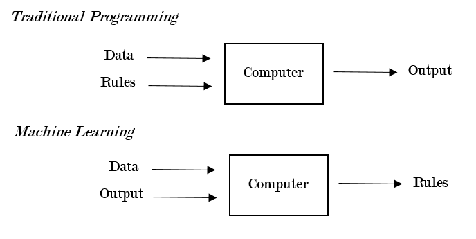
Figure 12.1: Traditional Programming v. Machine Learning
The first definition is by Arthur Samuel, a former researcher at IBM and early pioneer in machine learning. In his view, machine learning is a “field of study that gives computers the ability to learn without being explicitly programmed.” This definition is useful because it alludes to a central distinction between traditional programming and machine learning: i.e., in traditional programming, a computer takes in the data and the rules and generates the output; in machine learning, a computer takes the data and the output and generates the rules that describe the relationship between the input and the output. Figure 12.1 provides an illustration of this idea.
The second definition is more detailed and precise. According to Tom Mitchell, a computer scientist at Carnegie Mellon and the author of one of the first textbooks on machine learning: “A computer program is said to learn from experience E with respect to some task T and some performance measure P, if its performance on T, as measured by P, improves with experience E.” (Mitchell 1997). From the second definition, we can get a better sense of what machine learning generally entails: i.e., a computer gradually becomes better at performing a specific task (“what”) through experience (“how”); moreover, the computer’s performance is measured using some metric, which allows us to test whether performance has indeed improved over time. In this chapter, I will provide an overview of how machine learning methods work in practice and review some examples of how political scientists have used these methods in their research. Before proceeding, it is necessary to first explain several fundamental concepts in machine learning (for a more detailed treatment of this subject, see Hastie, Tibshirani, and Friedman 2017; James et al. 2013)
12.2 Background
12.2.1 A Brief Note on Notation
Capital letters refer to variables: e.g., \(Y\) refers to the outcome variable, such as vote choice. Lower-case letters refer to the observed value of the variable for a specific observation (or subject), denoted by the first subscript: e.g., \(y_{1}\) refers to the value of the outcome variable for the first observation. The subscript of a capital \(X\) refers to the number of the predictor or explanatory variable: e.g., \(X_{1}\) refers to the first predictor, \(X_{2}\) refers to the second predictor, and so on. In addition, \(x_{ij}\) refers to the observed value of the \(j\)th predictor for the \(i\)th observation. The ^ symbol indicates that we are referring to the predicted version or value of an object: e.g., \(\hat{f}(.)\) refers to an estimated function, \(\hat{Y}\) refers to the predicted value of the outcome variable.
12.2.2 The Structure of Prediction Error
Machine learning practitioners often talk about the best ways to \("\)minimize the mean squared error\("\) or \("\)optimize the bias-variance tradeoff.\("\) To understand how machine learning works, it is very important to understand the structure of prediction error. To illustrate, we can start with a simple example of a regression type problem with a quantitative outcome. Let \(Y\) be a 0-100 point feeling thermometer that measures attitudes toward the U.S. president, with 0 being very unfavorable and 100 being very favorable. Assume we are predicting \(Y\) using two predictors: ideology (\(X_{1}\)) and income (\(X_{2}\)). Formally, we can represent the relationship between \(X_{1}\), \(X_{2}\), and \(Y\) in the following way:
\[Y=f \left( X_{1}, X_{2} \right) + \epsilon\]
In the equation above, \({f}(.)\) is also known as the target function, which represents the true systematic (i.e., non-random) part of the relationship between the two predictors (\(X_{1}\), \(X_{2}\)) and the outcome \(Y\). On the other hand, \(\epsilon\) is the random error term, which is assumed to be independent of the predictors and have a mean of zero. In reality, of course, we do not know \({f}(.)\), so we have to estimate it using the data. Estimating the true function means that we are estimating the model’s parameters (e.g., the coefficients in a linear regression) or structure (e.g., the shape of a regression tree). For example, suppose we have a dataset (e.g., \(n\) observations) with the actual value of \(Y\), \(X_{1}\), and \(X_{2}\) for each observation: \(\{(y_{1},x_{11},x_{12}),...,(y_{n},x_{n1},x_{n2})\}\). Next, we will split the dataset into at least two parts, so that we can estimate \({f}(.)\) using one subset of the data (typically called the training set), and then evaluate the prediction error using the second subset of the data (typically called the test set).
Many machine learning algorithms are designed to estimate (or \("\)fit\("\)) a model that minimizes the expected prediction error (EPE), defined as the long-run average difference between the predicted and \("\)true\("\) (i.e., observed) values of the outcome variable. That is, the goal is to identify \({f}(.)\) such that \(f(X_{1},X_{2})\) is on average as close to \(Y\) as possible. How can we measure EPE in practice? When the outcome is a quantitative variable, the algorithms are often designed to minimize the mean squared error (MSE): i.e., the average of the squared difference between \(\hat{Y}\) and \({Y}\). The intuition here is that when the absolute difference between the predicted and observed values of the outcome variable is generally small, MSE will also be small.
\[MSE=\frac{1}{n} \sum _{i=1}^{n} \left( y_{i}-\hat{f} \left( x_{i1},x_{i2} \right) \right) ^{2}\]
Assuming we have split the original dataset into the training set and test set, we can compute two different types of MSE: training MSE and test MSE. In both cases, we first fit \(\hat{f}(.)\) using the training set. The difference, which is fundamental to machine learning, is the following: the training MSE (or training error, more generally) is then computed using the data from the training set, which contains the same data used to fit \(\hat{f}(.)\). In contrast, the test MSE (or test error) is computed using the test set, which was not used to fit \(\hat{f}(.)\).
Recall that we randomly assigned the observations in the original full dataset to the training and test sets. Thus, the two datasets are comparable: i.e., the true relationship between the set of predictors (\(X_{1}, X_{2}\)) and \(Y\) should be the same in both datasets. However, the two datasets are also not identical; these minor, non-systematic differences are due to random noise, which are represented by the \(\epsilon\) in Eq. 1. Given this context, it should be clear why we want to minimize test MSE instead of training MSE.
If we attempt to minimize training MSE, the algorithms are more likely to estimate highly flexible models that try to touch every data point in the feature space of the training dataset. This might initially sound nice, but it means that the model is overfitting to the training set: i.e., the model is attempting to capture both the real patterns due to the true \({f}(.)\), as well as the observed but spurious deviations from \({f}(.)\) that are due to the random noise (\(\epsilon\)). The problem here is that this kind of highly flexible model tends to generate a lower training MSE, but performs poorly on the test set—which has the same underlying patterns due to \({f}(.)\), but different observed deviations from \({f}(.)\) because of \(\epsilon\). Figure 12.2 provides an illustration of this idea. In this example, the true relationship between \(X_{1}\) and \(Y\) is linear (see the graph in the middle); we know this for certain because these data were simulated.
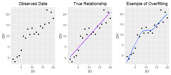
Figure 12.2: Modeling True Relationship v. Overfitting
Thus, it is a better idea to try and minimize test error. In order to generate a smaller test error, the algorithms need to estimate a model that is generalizable. That is, they need to estimate models that do a better job of capturing the true relationship between the set of predictors (\(X_{1},X_{2}\)) and the \(Y\), while ignoring the random observed deviations from the \({f}(.)\) due to \(\epsilon\) (per Equation 1). Machine learning practitioners often refer to this approach as \("\)focusing on the signal and ignoring the noise.\("\)
Check-in Question 1: What is overfitting and how can we reduce this problem?
So how do we reduce the test error? The expected difference between \(\hat{f}(X_{1},X_{2})\) and \(Y\) is due to two types of error (e.g., see James et al. 2013): (1) reducible error, (2) irreducible error. The first type of error is caused by a suboptimal estimate of the true function: i.e., the gap between \(\hat{f}(.)\) and \(f(.)\). As its name implies, the reducible error decreases as \(\hat{f}(.)\) approaches \(f(.)\). On the other hand, irreducible error is due to \(\epsilon\), and therefore it cannot be reduced by improving the quality of \(\hat{f}(.)\). For example, let us assume that \(\hat{f}(.) = f(.)\), and therefore \(\hat{Y} = \hat{f}( X_{1}+X_{2}) = f(X_{1}+X_{2})\). Even in this case, \(\hat{Y}\) does not necessarily equal \(Y\), because \(Y = f(X_{1}, X_{2}) + \epsilon\). That is, even having a perfect estimate of \(f(.)\) does not make the random error term go away.
Can we reduce \(\epsilon\)? The random error term represents omitted variables as well as truly random noise. If there are variables that are both useful predictors of \(Y\) and also largely independent of the existing predictors (\(X_{1},X_{2}\)), then by adding them into the model we can reduce \(\epsilon\). On the other hand, some of the \(\epsilon\) is ultimately due to random noise, and this component of \(\epsilon\) cannot be eliminated: e.g., perhaps some of the subjects felt particularly well/poorly the day they were surveyed, which affected how they responded to the survey questions.
To formally decompose the expected test error into its reducible and irreducible components, we can use the expected value (or long-run average) of the squared difference between \(\hat{Y}\) and \(Y\).20 The following proof requires knowledge of statistical theory (Larsen and Marx 2017; Rice 2007) and some basic algebra. To simplify the notation, let \(X=X_{1}+X_{2}\).
\[E \left[ \left( Y-\hat{Y} \right) ^{2} \right] =E \left[ \left( f \left( X \right) + \epsilon -\hat{f} \left( X \right) \right) ^{2} \right]\]
\[=E \left[ \left( \left( f \left( X \right) -\hat{f} \left( X \right) \right) + \epsilon \right) ^{2} \right]\]
\[=E \left[ \left( f \left( X \right) -\hat{f} \left( X \right) \right) ^{2}+2 \epsilon \left( f \left( X \right) -\hat{f} \left( X \right) \right) + \epsilon ^{2} \right]\]
\[=E \left[ \left( f \left( X \right) -\hat{f} \left( X \right) \right) ^{2} \right] +E \left[ 2 \epsilon \left( f \left( X \right) -\hat{f} \left( X \right) \right) \right] +E \left( \epsilon ^{2} \right)\]
\[=E \left[ \left( f \left( X \right) -\hat{f} \left( X \right) \right) ^{2} \right] +Var \left( \epsilon \right)\]
The first term, or the expected squared difference between \(\hat{f}(X)\) and \({f}(X)\), represents the reducible error. The second term, \(Var(\epsilon)\), represents the irreducible error. Although a full proof is beyond the scope of this chapter, note that we can further decompose the reducible error into squared bias and variance.
\[E \left[ \left( f \left( X \right) -\hat{f} \left( X \right) \right) ^{2} \right] = \left[ E \left( \hat{f} \left( X \right) \right) -f \left( X \right) \right] ^{2}+E \left[ \left( \hat{f} \left( X \right) -E \left( \hat{f} \left( X \right) \right) \right) ^{2} \right]\]
\[= \left[ Bias \left( \hat{f} \left( X \right) \right) \right] ^{2}+Var \left( \hat{f} \left( X \right) \right)\]
In sum, the expected test error (or expected prediction error, EPE) is a function of three specific quantities: the bias of \(\hat{f}(X)\), which indicates the gap between \(\hat{f}(.)\) and \(f(.)\); the variance of \(\hat{f}(X)\), which indicates how much \(\hat{f}(.)\) fluctuates depending on the training data; and \(Var(\epsilon)\), which is a measure of the non-systematic random noise in the data.
\[EPE=E \left[ \left( Y-\hat{Y} \right) ^{2} \right] = \left[ Bias \left( \hat{f} \left( X \right) \right) \right] ^{2}+Var \left( \hat{f} \left( X \right) \right) +Var \left( \epsilon \right)\]
The key insight is that the reducible error is itself a function of the squared bias and variance of \(\hat{f}(.)\), or the estimated model. Thus, to minimize the reducible error (and hence the total EPE), we want to minimize the bias and the variance.
Check-in Question 2: What is the expected prediction error (EPE), and why does it matter?
12.2.3 Bias-Variance Trade-offs
In machine learning, bias is a measure of the size of the gap between \(\hat{f}(.)\) and \({f}(.)\).21 The bias is smaller when the model does a better job of representing the true relationship between the set of predictors \((X_{1},X_{2},...,X_{p})\) and \(Y\). For example, let’s assume that the true relationship between \(X_{2}\) and \(Y\) is described using an inverted U-shaped curve. If the model we select imposes a linear functional form, then the bias will be larger than if the model allowed nonlinearity. Thus, to reduce bias, we often want to use a more flexible model.
However, it is possible for the model to be too flexible. Variance is a measure of the stability or consistency of the estimated model across training sets. If small changes to the training set (e.g., dropping a few observations) causes large changes in \(\hat{f}(.)\), then the variance is high. A highly flexible model tends to reduce bias but also increase variance (hence the idea of a \("\)trade-off\("\)). Thus, the goal is to fit a model that is flexible enough to capture the true relationship between the set of predictors \((X_{1},X_{2},...,X_{p})\) and \(Y\), but not so flexible that it is also fitting to the observed deviations from \({f}(.)\) in the training set due to \(\epsilon\).
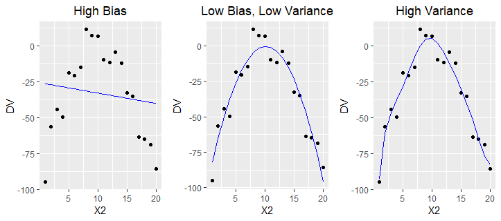
Figure 12.3: Bias-Variance Trade-offs
Figure 12.3 provides an illustration of this idea. The first model is not flexible enough, leading to high bias (also known as underfitting); on the other hand, the third model is too flexible, which leads to higher variance across slightly different training sets (overfitting). The second model imposes the ideal amount of flexibility, which optimizes the bias-variance trade-off and yields the smallest test MSE of the three alternatives.
Check-in Question 3: Explain why reducing bias can often entail an increase in variance.
12.2.4 Parametric v. Non-parametric Methods
Machine learning algorithms that make explicit assumptions about the functional form of the relationship between the set of predictors and \(Y\) are known as parametric methods. A well-known example is the ordinary least squares (OLS) regression. Given two predictors, \(f \left( X_{1}, X_{2} \right) = \beta _{0}+ \beta _{1}X_{1}+ \beta _{2}X_{2}\). Thus, the regression equation in this case can be written as follows:
\[Y= \beta _{0}+ \beta _{1}X_{1}+ \beta _{2}X_{2}+ \epsilon\]
Parametric methods offer several key advantages. First, they simplify the task of estimating \(f(.)\) by making an assumption about the functional form or shape of \(f(.)\). In the case of an OLS regression, the algorithm assumes that \(f(.)\) is linear with respect to the parameters (i.e., the coefficients and the error term), although not necessarily with respect to the values of the predictors. Thus, the only task is to estimate coefficients: \(\beta _{0}, \beta _{1}, ..., \beta _{p}\). Second, because of the functional form assumption, the \(\hat{f}(.)\) tends to be more stable across comparable training sets (i.e., lower variance); put differently, the estimated model is more robust to minor fluctuations due to \(\epsilon\). Another advantage is that parametric methods also tend to score high on interpretability: e.g., we can easily interpret \(\beta _{1}\) as indicating that a one-unit change in \(X_{1}\) is associated with a change of \(\beta _{1}\) in \(Y\). Other examples of parametric methods include logistic regression, penalized regression methods (e.g., lasso, ridge), and linear discriminant analysis. The main disadvantage of parametric methods is the risk of imposing a functional form that is very different from the true \(f(.)\), which can result in higher bias (or more prediction error). We can mitigate this risk by adjusting the parametric methods so that they are more flexible (e.g., by using higher-order terms in an OLS regression), but this may come at the cost of higher variance.
Non-parametric methods do not assume that the true relationship between a set of predictors and \(Y\) follows a specific functional form; instead, they inductively attempt to estimate \(f(.)\) such that it closely follows the training observations in the feature space. Well-known examples of non-parametric methods include tree-based methods (e.g., random forests, boosted trees), support vector machines (SVM), and K-nearest neighbor (KNN). The main advantage of non-parametric methods is that by design, they are very flexible; this means that they can be particularly useful when the relationship between the predictors and the outcome is highly complex. In such cases, non-parametric methods can outperform parametric methods by achieving lower bias, and ultimately, lower test error.
However, non-parametric methods also have a number of disadvantages. Since they do not make assumptions about the functional form, they often require much larger training sets in order to estimate \(f(.)\). In addition, because they are highly flexible, non-parametric methods may also be subject to higher variance across training sets due to overfitting. This can be mitigated by properly tuning the models using cross-validation (CV), a model selection procedure discussed later in this chapter. Finally, it is also often more difficult to interpret the nature of the relationship between a specific predictor (e.g., \(X_{1}\)) and the outcome. This is why some especially complex non-parametric methods such as artificial neural networks (ANN) are often called \("\)black box algorithms,\("\) since it is not clear exactly how the \(f(.)\) is being estimated.
Given this discussion, which methods are preferred? It depends on the size of the available data, the complexity of the relationships among the variables, and the goals of the method. Machine learning practitioners are often interested in prediction or (causal) inference. If the goal is prediction, then we are less concerned about understanding the specific nature of \(f(.)\). Instead, we are satisfied as long as we can estimate a model such that \(\hat{f}(X) \approx Y\). In this case, we should choose the parametric or non-parametric method that generates the lowest expected test error. On the other hand, if we are interested in understanding the specific nature of the relationship between a given predictor (or group of predictors) and the outcome, it may make more sense to select a parametric method, which produces results (e.g., regression coefficients) that are easier to interpret. While social scientists are often more interested in causal inference than prediction alone, they have used both parametric and non-parametric methods in their research. Several examples from political science will be discussed later in this chapter.
12.2.5 Supervised v. Unsupervised Learning
We can also classify machine learning methods according to whether they predict a specific outcome. In supervised learning, there is a clearly defined \("\)correct answer\("\) – and the purpose of the machine learning algorithm is to correctly predict that answer. For instance, let us assume we want to predict whether a U.S. citizen will vote in the next presidential election. This is an example of a supervised learning problem; since the person either will or will not vote, there is clearly a \("\)correct answer.\("\) There are two types of supervised learning, which are distinguished by the type of outcome predicted: (1) regression, (2) classification. In regression, the goal is to predict a continuous or quantitative outcome: e.g., test scores, stock prices, inflation rates, number of children, and so on.22 In classification, the goal is to predict a categorical or discrete outcome: e.g., religion, political party membership, vote choice, occupation, whether a person holds a four-year degree.23
In unsupervised learning, the purpose of the machine learning algorithm is to examine the underlying structure of the data and identify \("\)hidden\("\) patterns. It is not attempting to correctly predict an outcome. One well-known example of an unsupervised learning method is clustering: clustering algorithms (e.g., hierarchical, k-means) identify latent groups of observations by examining the relationships among the variables associated with the observations (Bryan 2004; Wagstaff and Cardie 2000; Witten 2011). In this case, we do not know ahead of time what the \("\)correct\("\) or \("\)true\("\) number of clusters is. Researchers can use clustering algorithms to identify more internally homogeneous groups of subjects (e.g., with respect to demographic characteristics, attitudes, preferences, consumption patterns). Figure 12.4 provides an illustration of how we may organize machine learning methods by type and subtype. Please note that the list of examples is not meant to be exhaustive.
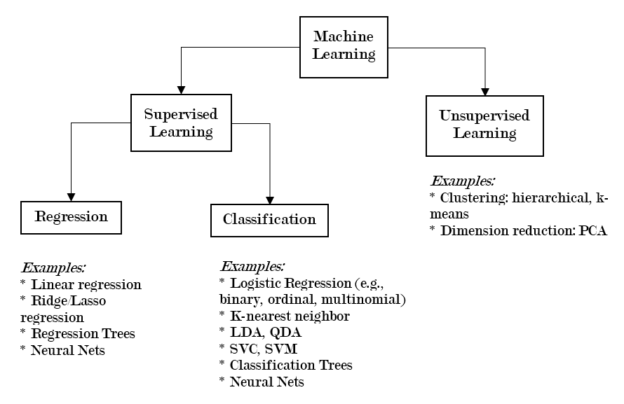
Figure 12.4: Types of Machine Learning Methods
Check-in Question 4: What is the main difference between supervised and unsupervised learning?
12.3 Method: setup/overview
There are definitely variations in how researchers and other practitioners organize their machine learning projects. However, the workflow tends to follow a general pattern. Assuming you already decided to use one specific method (e.g., lasso regression), the workflow may look something like this:
Split the data into training and test sets
With just the training set, use k-fold cross-validation (CV) to perform model selection (i.e., optimize the tuning parameters)
Fit the final optimized version of the model (also called the candidate model) using the full training set
Assess the candidate model by computing the test error
If you would like to compare the performance of multiple methods (e.g., boosted trees, random forests), then only a few modifications to the sample workflow above are necessary. Repeat steps 2-4 for each of the methods. At the final stage, you will have the test error for each candidate model: depending on your ideal trade-off between accuracy and interpretability, you can then select the most preferred model. For example, if the goal is causal inference, then you may be willing to select the candidate model with a somewhat higher test error because it scores much higher on interpretability.
12.3.1 What is Model Selection?
The performance of machine learning models is often highly dependent on their tuning parameters. We can think of tuning parameters as levers of the model that allow us to customize or adjust how it operates. Model selection refers to the process of identifying the tuning parameters that yield the lowest expected test error; this is also referred to as \("\)optimizing the tuning parameters.\("\) For example, consider the lasso regression, which is a powerful method when we know that most of the predictors are probably not useful for predicting the outcome. If a normal OLS regression is used in this situation, the coefficients that should actually be zero may remain at non-zero values—which increases the likelihood of the model overfitting to the training data.
The algorithms for the OLS and lasso regressions are similar, except that the optimization process for the latter is subject to an additional constraint. Basically, this extra constraint imposes a penalty for the sum of the coefficients for the \(p\) predictors in the model. The size of the penalty is controlled by \(\lambda\): the bigger the \(\lambda\), the smaller the coefficients. In fact, when the \(\lambda\) is sufficiently large, many of the coefficients are totally zeroed out, which means that the lasso regression also provides a means of automating the variable selection process. Next, I explain why we typically use a method known as \(k\)-fold cross-validation to perform the model selection procedure.
\[\lambda \sum _{j=1}^{p} \vert \beta _{j} \vert\]
12.3.2 Why K-Fold Cross-Validation?
For example, let us assume that we want to compare 100 unique values of \(\lambda _{i}\) for the lasso regression; how do we know which value will yield the lowest test error rate?
One option is using the validation set approach. This entails randomly splitting the training set (\(n_{1}\)) into two non-overlapping subsets: a model-building set (\(n_{1a}\)) and a validation set (\(n_{1b}\)). Next, we fit a model using the model-building set (\(n_{1a}\)) and the first value of lambda (\(\lambda _{1}\)), and then test it against the validation set (\(n_{1b}\)). We would then repeat this process 99 more times, so that we have done it once for each \(\lambda _{i}\). Afterward, we could compare the 100 validation error rates and identify the value of the parameter that generated the lowest validation error. However, this approach has two important disadvantages (James et al. 2013, 176–78). First, the estimated validation error rate for each \(\lambda _{i}\) is highly variable, since it is very sensitive to the specific observations that were randomly selected to be in \(n_{1a}\) and \(n_{1b}\); if a small percentage of the observations in the \(n_{1a}\) were moved to \(n_{1b}\) (and vice-versa), the test error rate would likely change. Second, statistical learning models tend to perform more poorly when trained on a smaller dataset; thus, by only training the model on a subset of the full training set (i.e., since \(n_{1a} \ll n_{1}\) ), we may actually overestimate the test error.
\(K\)-fold cross-validation (CV) is a statistically efficient resampling method that addresses both of these problems. The purpose of CV is to provide a more reliable estimate of the test error, which can then be used to compare and evaluate unique values of the tuning parameters (e.g., \(\lambda _{i}\)). It involves randomly splitting the training set (\(n_{1}\)) into \(k\) non-overlapping groups (or \("\)folds\("\)) that are equal in size; the first fold is treated as the held-out validation set, and the model is fit using the observations in the remaining \(k-1\) folds. This process is repeated until each fold has served as a validation set.
If there are 10 folds, there are also 10 estimates of the validation error; these estimates are averaged to form the CV error rate. The idea is that this CV error rate is a more reliable estimate of the validation error since it is based on an average of \(k\) estimates (i.e., the CV error rate has a lower variance). Returning to the previous example, if we wanted to test 100 potential values of \(\lambda _{i}\), we would perform the \(k\)-fold CV procedure for each \(\lambda _{i}\); then, we would choose the value of \(\lambda _{i}\) that yielded the lowest CV error.
12.4 Method: detail
In this section, I provide a brief overview of two common classes of machine learning methods, and how they actually work in practice: (1) tree-based methods, (2) support vector machines. Since we have used quantitative outcomes so far in our examples, this time the examples will focus on classification: 1 = voted for Trump in 2016, 0 = voted for someone else.
12.4.1 Model Class: Tree-based Methods
All tree-based methods (e.g., bagged trees, random forests, boosted trees) share some important similarities. Each tree divides the training observations into \(m\) non-overlapping regions of the predictor space \(\{ R_{1},R_{2}, \ldots R_{m} \}\). Internal nodes refer to the place where the splits are made. The algorithm uses binary recursive splitting, and generally operates in the following way. The splits (i.e., predictor used, values of the predictor) are chosen in order to maximize the purity or homogeneity of the child nodes with respect to outcome class: i.e., in this case, whether or not the respondents voted for Trump (i.e., \(Vote=1\) or \(Vote=0\)). As such, the first split has the most explanatory power (i.e., in terms of being able to predict the outcome class of a training observation), the second split has the second most explanatory power, and so on.
Node purity or homogeneity is often measured using the Gini index or entropy. In both cases, the measures are smaller when the nodes (or regions) are more homogeneous; thus, the objective is actually to choose splits that minimize the Gini index or entropy (which is equivalent to maximizing node purity). The Gini index is defined below (James et al. 2013, 312). Here, \(p_{mk}\) represents the proportion of the training observations that are in \(m\)th region (\(R_{m}\)) from the \(k\)th class. Recall that \(G\) is small when the nodes are more homogeneous: e.g., when the proportion of training observations in \(m\)th region are closely split between two classes \(45\% -55\%\), then \(G = (.45)(.55)(2) =0.495\); in contrast, when the training observations in \(R_{m}\) are more dominated by a single class (and thus \(R_{m}\) is more homogeneous), for instance, \(90\% -10\%\) , then \(G = (.10)(.90)(2) = 0.18\).
\[G= \sum _{k=1}^{K}p_{mk} \left( 1-p_{mk} \right)\]
How does this work in practice? For example, let us assume that in the training set, being white v. not being white was the strongest individual predictor of the Trump vote (i.e., it would maximize node purity). If this were the case, then the first split would be based on race: all white respondents would be assigned to the right branch, and all non-white respondents would be assigned to the left branch (see Figure 12.5 below). Next, let us assume that among white respondents, being above the mean on the 1-7 point political conservatism scale is the strongest predictor of the Trump vote; if so, then the second split would be based on whether the white respondents’ conservatism score is \(\leq 4.3\) (left branch) or \(> 4.3\) (right branch).
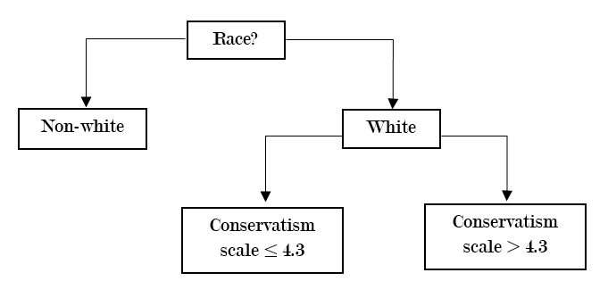
Figure 12.5: Example of a Decision Tree
In this simple example, the observations (or respondents) in the training set are assigned to one of three non-overlapping regions in the predictor space: \({R_{1}= \{Vote \vert minority}\}\), \(R_{2} = \{Vote \vert white, conservatism \leq 4.3\}\), and \(R_{3}= \{Vote \vert white, conservatism > 4.3 \}\). To predict the outcome class of an observation in the validation or test set, we simply look at which region the observation would be assigned to based on its predictor values (e.g., is \(x_{1} = white\)?), and then choose the most common class of that region. For instance, if the test observation would belong to \(R_{3}\), and \(70\%\) of the training observations in \(R_{3}\) voted for Trump, then the predicted class of that test observation would be \(Vote=1\). In general, of course, there are usually more than three regions (or terminal nodes); the splitting ends once a stopping point is reached: e.g., in order to satisfy the minimum terminal node size.
Individual decision trees suffer from high variance: i.e., the structure of the tree is highly dependent on which specific observations randomly end up in the training set. To address this issue, we can use the average prediction of many different trees. Methods for combining these different trees are called decision tree ensembles. There are three popular approaches: bagging24, random forests25, and boosting26
12.4.2 Model Class: Support Vector Machines
Support Vector Machines (SVMs) are a class of methods that seek to assign observations to the correct outcome by using hyperplanes as decision boundaries. Hyperplanes are a \(p-1\) dimensional flat subspace in a \(p\)-dimensional space: e.g., if \(p = 2\) (there are 2 predictors), then the hyperplane is simply a line. For instance, let us assume a simple case in which we are predicting the binary outcome \(Vote\) using only two predictors; in this case, the separating hyperplane is a line. If the respondents in the training set who voted for Trump are labeled as \(y_{i}=1\), and those who did not vote for Trump are labeled as \(y_{i}=-1\), then the separating hyperplane can be formally described as follows:
\[y_{i} \left( \beta _{0}+ \beta _{1}x_{i1}+ \beta _{2}x_{i2} \right) >0\]
In this case, when \(\beta _{0}+ \beta _{1}x_{i1}+ \beta _{2}x_{i2}>0\), \(y_{i}=1\) and if \(\beta _{0}+ \beta _{1}x_{i1}+ \beta _{2}x_{i2}<0\), then \(y_{i}=-1\). That is, we can classify the observations based on whether they are above or below the separating hyperplane.
Next, I will briefly review how SVMs have been designed to address two key practical challenges. The first challenge is that there are often many hyperplanes that can correctly classify the observations, since the hyperplane can be slightly adjusted in any direction and probably still produce the same classifications. If we return to the equation above, it is easy to see that there are many ways the coefficients \(\beta {0}\), \(\beta {1}\), and \(\beta {2}\) can be slightly adjusted (e.g., a \(0.5\%\) increase or decrease) and still perfectly classify the observations. The solution is to maximize the margins, or the distance between the training data points and the separating hyperplane: this is also known as the maximal margin classifier or MMC.
Unfortunately, the MMC approach faces its own problems. Sometimes, there is simply no perfectly separating hyperplane; and even if there is, it is highly sensitive to individual observations, which can lead to overfitting (and high variance). The solution is a more flexible form of the MMC that allows some observations to fall on the wrong side of the margin and/or hyperplane: this is also known as the support vector classifier (SVC). The SVC is more robust in that it is less sensitive to individual observations, such as outliers (i.e., since some violations of the margin are allowed); this property allows the SVC to do a better job of classifying the observations in general.
Like the MMC, the SVC seeks to maximize the margin, but it is subject to a number of important constraints (James et al. 2013, 346–47). Here, I will specifically focus on the cost parameter (\(C\)), since that is what is generally optimized using cross-validation. Below, \(\epsilon {i}\) indicates how severely the \(i\)th observation violates the margin and separating hyperplane. When \(\epsilon {i}=0\), the \(i\)th observation is located on the correct side of the margin (i.e., no error); when \(\epsilon {i}>0\), it is on the wrong side of the margin; and if \(\epsilon {i}>1\), it has actually violated the separating hyperplane. That is, \(C\) essentially represents the budget for the number and severity of the classification errors across the \(n\) observations. When \(C\) is small, the SVC will fit more tightly to the training observations in the feature space, at the cost of higher variance; and when \(C\) is large, the opposite can occur. To optimize this bias-variance trade-off, we can use k-fold CV.
\[\sum {i=1}^{n} \epsilon {i} \leq C\]
The SVM is an extension of the SVC, which allows us to model nonlinear decision boundaries using kernels. By using kernels, the SVM allows us to expand the feature space (e.g., include polynomial functions of the predictors) in a computationally efficient manner. For more details on this procedure, we can refer to James et al. 2013, pp. 350-353; and Hastie et al. 2017, pp. 423-426).
12.5 Applications
In this section, I review six recent examples of machine learning methods in political science articles. The examples cover applications of both supervised learning (e.g., RF, SVM, naïve Bayes, k-nearest neighbor); and unsupervised methods such as topic modeling, which is related to clustering. Several different subfields of political science are represented: U.S. politics, political theory, comparative politics, international relations, and peace and conflict studies; in addition, the articles use data from many countries around the world (e.g., Argentina, India).
12.5.1 Example 1: U.S. Politics
DW-NOMINATE scores are often used in political science as a measure of a legislator’s ideology; they are based on the actual votes the legislators have made on bills in the U.S. House or U.S. Senate. uses two supervised machine learning methods (i.e., support vector regression and random forests) to address a very interesting problem: how can we predict the ideology of new legislators before they begin casting their votes? Support vector regression (SVR) is very similar to SVM, except that the algorithm has been modified to enable the prediction of a continuous outcome. In the first part of the paper, the author uses 10-fold CV to train models that predict the candidates’ DW-NOMINATE scores based on their campaign contributions, gender, party, and home state. The training set includes candidates with DW-NOMINATE scores between 1980-2014; and the key predictors in the feature matrix are the names of donors who have given to at least 15 candidates (e.g., National Education Association).
According to the results (i.e., RMSE),27 the support vector regression and random forest methods perform at least as well as the other methods that actually use the roll call data. This is especially impressive when we consider that the roll call data are used to construct the DW-NOMINATE scores. Next, Bonica also shows that the supervised learning methods also do a very good job of correctly predicting the actual votes cast during the 96th-113th Congresses: e.g., 89.9\(\%\) of the votes are correctly predicted using DW-NOMINATE, which is not surprising; however, 89.5\(\%\) and 89.3\(\%\) of the votes are also correctly classified using the RF and SVR methods that were only trained using campaign contributions and a few other predictors.
12.5.2 Example 2: Comparative Politics
How do we know whether an election was rigged? Using synthetic (i.e., simulated) data, Cantú and Saiegh (2011) train a naïve Bayes classifier that successfully identifies fraudulent elections in the Buenos Aires province of Argentina between 1931 and 1941. One of the greatest strengths of the naïve Bayes (NB) algorithm is its simplicity, which is due the assumption that the features (i.e., predictors) are independent.28 For every election, the algorithm first estimates the posterior probability of membership in each class (i.e., fraudulent or clean) given the set of observed features or attributes associated with the election. The predicted class of each election is the class with the largest posterior probability, per Bayes theorem. For example, given a set of features, if the election is even slightly more likely to be fraudulent than clean, the election is classified by NB as a fraudulent election, and vice versa. After training their NB classifier on a large synthetic dataset (N=10,000), the authors test their model using several well-documented elections in 1936, 1940, and 1941; they show that their method ultimately outperforms key existing fraud detection algorithms (e.g., those based on the distributions of digits in official vote counts).
12.5.3 Example 3: Political Theory
Can machine learning be used to study the evolution of political theory across centuries? During the medieval and early modern period, scholars and other elites often wrote advice books for leaders that covered topics such as military strategy, economic prosperity, and religious devotion. These books provide an insightful view or \("\)mirror\("\) into the dominant political theories and paradigms of the day. Blaydes, Grimmer, and McQueen (2018) use automated text analysis to compare how political advice texts in the Medieval Christian and Islamic Worlds changed during the medieval period. Their corpus of text includes 21 texts from the medieval Islamic world, which were produced between the eighth to seventeenth centuries; and 25 texts from Christian Europe, which were produced between the sixth to seventeenth centuries. Specifically, the authors use a hierarchical form of topic modeling based on variational approximation; while topic modeling methods vary in their specific details, all of them are unsupervised learning methods that seek to identify latent or \("\)hidden\("\) clusters of topics in bodies of text (Wallach 2006).
Blaydes et al. identify four broad themes and 60 specific sub-themes nested within the broader themes; the four broader themes include: being a good ruler, the personal virtues of rulers, religion, and political geography or space. A key finding of the study is that at the aggregate level, the Christian and Muslim texts generally allocated a similar share of the space for each of the four broad topics. For example, topic 1 was the most prevalent issue across both Christian and Muslim works. However, there are some differences in trends across time. Whereas the prevalence of religious content steadily declined during the medieval period in Christian works, a similar temporal trend was not observed for advice books published in the Islamic world. The authors provide an interesting discussion of what these findings may mean for how we understand the relationship between political theory and institutional development.
12.5.4 Example 4: Comparative Politics
In a very recent study, Parthasarathy, Rao, and Palaniswamy (2019) use natural language processing (NLP) and topic modeling to study deliberative processes in the rural villages of South India. Their dataset includes a corpus of transcripts from a geographically representative sample of 100 village assemblies (or \("\)gram sahbas\("\) ) in Tamil Nadu, a state in southern India. Parthasarathy and her coauthors use an unsupervised topic learning approach called structural topic modeling (STM), which identifies clusters of co-occurring words in the corpus of text. They identify 15 topics, with the most popular topics being water, beneficiary and voting lists, and employment and wages. By combining these topics with the use of statistical tests, the authors show that female participants face serious inequalities: “Women are less likely to be heard, less likely to drive the agenda, and less likely to receive a relevant response from state officials” (pp. 637-638). For example, politicians provided a relevant (i.e., on-topic) response to women only 49\(\%\) time, but to male speakers 70\(\%\) of the time. These disparities are problematic not only because they indicate that female voices tend to matter less in deliberative processes, but also because the issues that disproportionately affect women may be less likely to be translated into meaningful policy outputs.
12.5.5 Example 5: Peace and Conflict
In a fascinating paper, Mueller and Rauh (2018) combine a number of methods (i.e., topic models, lasso regression, linear fixed effects models) to predict political violence using newspaper text. First, they downloaded 700,000 newspaper articles about events in 185 countries from the New York Times (NYT), the Washington Post (WP), and the Economist. All available articles published between 1975-2015 were included in the text corpus. Topic modeling based on Dirichlet allocation (LDA) is used to reduce the high dimensionality of the text corpus (i.e., almost a million unique words, after preprocessing) to 15 topics. The relative prevalence of each topic is aggregated at the level of country-year and used as predictors in linear fixed effects models. The results show that the within-country variation over time in topic prevalence is a robust predictor of the outbreak of civil war and armed conflict: the area under the curve (AUC) indicates that about 73-82\(\%\) of the outcomes can be correctly predicted using only within unit variation. The authors also use lasso regressions, an automated variable selection method, to identify the most important predictors: e.g., the prevalence of the \("\)justice\("\) topic is a significant predictor of political violence across several different values of lambda, the penalty parameter. This finding is substantively important because it reinforces the idea that institutional design, the rule of law, and social stability are often tightly coupled together in reality.
12.5.6 Example 6: International Relations
Although power is a key concept in international relations, there is no consensus over the best way to measure it. Carroll and Kenkel (2019) use machine learning to develop a new method of measuring power, called the Dispute Outcome Expectations (DOE) score. To create the DOE scores, they used a two-step process: first, a number of machine learning methods (e.g., SVM, k-nearest neighbors, RF, neural nets) were used to predict the outcomes of militarized international disputes between 1816 and 2007. Then, a super learner algorithm was used to combine the results and create an optimal weighted ensemble of the models. Carroll and Kenkel demonstrate that the DOE does a much better job of predicting the probability of conflicts between two states (called dyads) than the national capability ratio, which is frequently used in the literature. Using this superior measure of power also improves our substantive understanding of the nature of interstate conflict: the probability of interstate conflict is the greatest when there is a large disparity in power and the more powerful state does not prefer the status quo—a finding that seems more sensible and in line with existing theories.
12.6 Advantages of Method
What are the advantages and disadvantages of machine learning, especially in the context of the social sciences? The advantages are considerable. Machine learning algorithms can increase prediction accuracy, which is especially important when we are attempting to predict highly consequential outcomes (e.g., outbreak of violent conflicts). They can also reduce the effects of human biases, by automating many decisions (e.g., variable selection); in addition, modern machine learning methods are also very computationally efficient (e.g., due to vectorization), which means that truly vast amounts of data can be analyzed.
12.7 Disadvantages of Method
However, machine learning methods also face some disadvantages. To accurately predict the outcomes of highly complex or contingent processes, large amounts of data are often necessary but sometimes unavailable; classification methods (e.g., classification trees, SVM) tend to perform poorly when the classes are imbalanced; many algorithms are prone to overfitting; and gains in prediction accuracy can sometimes come at the cost of reduced interpretability. In addition, machine learning methods may also generate results that seem socially undesirable or biased against certain groups. While these challenges are very real, many of them can be addressed by existing best practices as well as future innovations. For example, using k-fold cross-validation can help reduce overfitting and optimize the bias-variance trade-off; we can also minimize the risk of \("\)biased algorithms\("\) by remaining cognizant of the biases or problems that may be present in the training data.
12.8 Broader significance/use in political science
As evidenced by the examples discussed above, machine learning methods are broadly applicable across the social sciences (Mason et al. 2014). You are more likely to see them used when there are a lot of data, the relationships among variables are highly complex, and the key patterns in the data are not obvious to the human eye. Political scientists have successfully used machine learning methods (e.g., k-fold CV) and algorithms to pursue research questions in subfields including U.S. politics, comparative politics, international relations, and political theory. For instance, political scientists frequently use unsupervised learning methods such as topic modeling to automate the analysis of large bodies of text. In recent years, researchers have also been increasingly using multiple machine learning models in the same project (e.g., topic modeling and linear regressions), in order to address more complex research questions or gain more prediction accuracy.
12.9 Conclusion
The era of \("\)big data\("\) has arrived. Large technology companies such as Amazon, Apple, Facebook, Google, and Twitter are harvesting unprecedented amounts of data from their users across the globe. At the same time, political scientists and other social scientists (e.g., economists, sociologists) are interested in advancing our understanding of the social world. Why do people choose to vote (or not vote)? Under what conditions will countries go to war with each other? What makes some proposed bills more likely to be passed into law? This is an exciting time for quantitative social science research. Recent advancements in machine learning, while not without their challenges, offer many new and exciting ways to analyze an increasingly large quantity and variety of data. If handled properly, the findings generated from these new methods could improve our understanding of complex social processes, inform policymakers, and improve human societies.
12.10 Application Questions
Imagine you are the director of analytics for a U.S. Senate candidate. Briefly describe how you could use a machine learning method in your work. Why did you choose this method? What are some advantages and disadvantages of the method you chose?
Imagine you are a consultant and your client is a federal law enforcement agency that wants to predict the likelihood of a violent protest in various regions of the country. Briefly describe how you could use a machine learning method in your work. Why did you choose this method? What are some advantages and disadvantages of the method you chose?
12.11 Key Terms
- target function
- training set
- test set
- expected prediction error (EPE)
- training error
- test error
- overfitting
- underfitting
- reducible error
- irreducible error
- expected value
- bias
- variance
- bias-variance trade-offs
- parametric methods
- non-parametric methods
- model interpretability
- model flexibility
- k-fold cross-validation
- prediction v. (causal) inference
- supervised v. unsupervised learning
- regression v. classification methods
- model selection
- candidate model
- tuning parameters
- validation set approach
12.12 Answers to Application Questions
There is no single correct answer. However, for both questions, a strong answer will specify the method type (e.g., supervised, regression v. classification) and discuss issues such as the bias-variance trade-off, cross-validation, model interpretability, and prediction accuracy.
References
Here is a more detailed explanation of what is meant by this sentence. The squared difference between \(Y\) and \(\hat{Y}\) is actually a continuous random variable. In statistical theory, a random variable is a variable whose value is the outcome of a random process. Recall that in the general case \(Y = f(X) + \epsilon\), where \(X\) represents a set of predictors. Since \(Y\) is the function of the random error component \(\epsilon\), \(Y\) is by definition a random variable. Now, notice that since \((Y-\hat{Y})^{2}\) is a function of the random variable \(Y\), \((Y-\hat{Y})^{2}\) must also be a random variable. In particular, \((Y-\hat{Y})^{2}\) is a continuous random variable, since it can theoretical take on an infinite number of possible (non-negative) values. We can think of the expected value of a random variable as being the weighted or “long-run” average of the random variable’s possible values. To simplify the notation, let \(W=(Y-\hat{Y})^{2}\). Formally, let’s assume that the random variable \(W\) has a probability density function \(g(w)\), which determines the distribution of the probabilities associated with the possible values of \(W\). The lower-case \(w\) represents specific possible values of the random variable \(W\). In this case, then \(E(W) = \int_{-\infty}^{\infty} wg(w) dw\).↩︎
Another way to think about bias is that it is the systematic part of the difference between \(Y\) and \(\hat{Y}\). When \(\hat{f}(.)\neq{f}(.)\), the observed difference between \(Y\) and \(\hat{Y}\) is often correlated with the gap between the estimated function and the true function.↩︎
Examples of popular supervised learning methods for regression include the ordinary least squares (OLS) regression, penalized/shrinkage methods such as the ridge and lasso regressions, regression trees, and artificial neural networks (ANN).↩︎
Examples of popular supervised learning methods for classification include various implementations of the logistic regression (i.e., binary, ordinal, multinomial), k-nearest neighbor (KNN), linear discriminant analysis (LDA), quadratic discriminant analysis (QDA), support vector classifiers (SVC), support vector machines (SVM), classification trees, and artificial neural networks (ANNs).↩︎
This entails creating \(B\) bootstrap samples by sampling with replacement from the original training set (\(n_{1}\)). A classification tree is fit using each sample, and then the trees are combined (Cutler et al. 2014). This method is superior to using a single decision tree, because a single decision tree is affected by high variance; in contrast, by averaging the predictions across many \(B\) trees, the variance is reduced. The main tuning parameter for bagged trees is \(B\), the number of bootstrapped trees.↩︎
This is the same as bagging, but now the model is only allowed to consider only a random subset \(m\) of the \(p\) predictors at each split (such that \(m \ll p\), e.g., \(n \approx \sqrt{p}\)). The logic here is that by intentionally restricting the number of predictors that can be considered at each split, the trees will become less correlated (Cutler 2005). In many cases, decorrelating the \(B\) trees in this way can lead to reduced test error.↩︎
With boosted trees, the trees are grown sequentially: each tree is fit to the residuals from the previous model. The logic of this approach is that it allows each successive tree to address the weaknesses of the previous tree.↩︎
Root mean squared error (RMSE) is a measure of the average absolute difference between the predicted value of the outcome and the actual observed value. The smaller the RMSE, the more accurate the estimates of the outcome.↩︎
Although this is a strong assumption, research has shown that NB algorithm is robust to minor deviations from independence of the features.↩︎